It is common to use footnotes when reporting financial results. Footnotes allow you to be transparent with the viewer and disclose important assumptions or clarifications so that they can more accurately interpret the results. By using superscript numbers, we can make adding footnotes to financial reports and charts in Excel easier.
To create a superscript number in Word or PowerPoint, you can select the specific number and use the font formatting feature to make just the selected text superscript. If you select one character in a text string in the formula bar in Excel, you can use the full font dialog box to make that one character superscript.
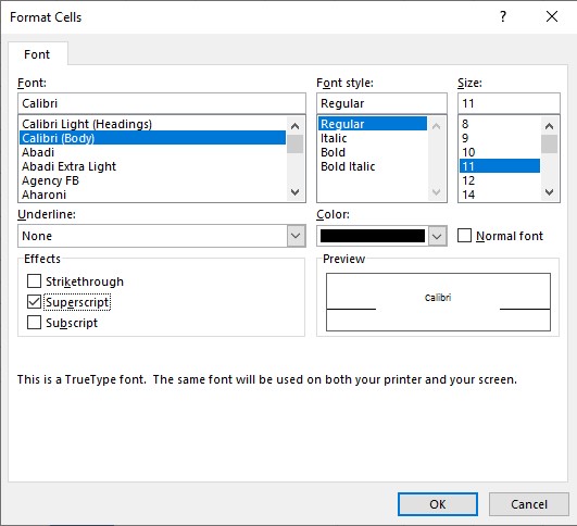
This technique will not work if the cell is a number even though it may appear to do so initially. When you confirm the editing by pressing the Enter key, the superscript format is removed.
To make the use of superscript numbers for footnotes more flexible, I want to show you how to create text strings that include superscript number using functions. This will allow you to create text strings to use in cells, chart titles, or chart data labels if you want.
Superscript numbers can be created using the CHAR and UNICHAR functions in Excel. Here is a list of which function to use to create superscript numbers.
| Superscript Number | Function |
| 1 | CHAR(185) |
| 2 | CHAR(178) |
| 3 | CHAR(179) |
| 4 | UNICHAR(8308) |
| 5 | UNICHAR(8309) |
| 6 | UNICHAR(8310) |
| 7 | UNICHAR(8311) |
| 8 | UNICHAR(8312) |
| 9 | UNICHAR(8313) |
Here are three examples of using superscript numbers for footnotes.
Example #1: In a table of cells
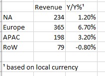
When you want one cell to contain a superscript number, use the text concatenate operator (&) to join strings together. If the cell contains text, the formula could be =”Y/Y%”&CHAR(185).
If the cell is a number, you can’t add the superscript in the same cell or any calculations using that cell will cause an error. Instead, place the superscript in the cell to the right of the cell containing the number and left align the text. This may require a new column just to contain the superscript number.
For the cell with the footnote explanation, use a similar formula to concatenate the superscript number and the explanation text. Typically this footnote cell is placed below the cells containing the numbers or text that have the footnote reference.
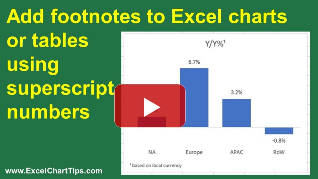
Example #2: In a chart title
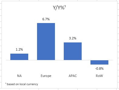
If you have typed the chart title in, you can use the method at the start of the article to make one character in the text superscript.
You can also use a formula that includes a superscript number and the chart title text to create a cell that is used as the chart title. If you only have one data series in a basic column chart, Excel may use the series name as the chart title by default instead of a legend. The formula with the superscript number can be used to create the data series name in this case.
The footnote text in the example above is created by using the horizontal axis title in the chart. The horizontal axis title is added to the chart and is set to use a cell in the worksheet that contains a formula using the superscript number and the footnote explanation. The axis title is then dragged to the lower left corner of the chart area.
Example #3: In a chart data label
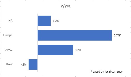
If the footnote only applies to one data point, you can use the feature that was introduced in Excel 2013 to add data labels from a different set of cells. Create a set of cells that contains text strings of the values using the TEXT function to format the numbers. To the one data label that requires the footnote, concatenate the superscript number using the function for that number.
When you add data labels to the data series, use the Value From Cells option and select the range of cells you created.
The footnote in the example above is created using a text box added on top of the chart and is set to use a cell in the worksheet that contains a formula using the superscript number and the footnote explanation. The text box is then dragged to the lower right corner of the chart area. Text boxes are not as flexible as using the horizontal axis title option as shown in the previous example. They do not automatically resize if the chart is resized and require more manual sizing to ensure that all the text appears.
To give yourself maximum flexibility when using footnotes in Excel reporting, use the functions in the table earlier to add superscript numbers to text cells that can be used below cells or as part of an Excel chart.
Below is a video that shows these techniques in Excel.

Dave Paradi has over twenty-two years of experience delivering customized training workshops to help business professionals improve their presentations. He has written ten books and over 600 articles on the topic of effective presentations and his ideas have appeared in publications around the world. His focus is on helping corporate professionals visually communicate the messages in their data so they don’t overwhelm and confuse executives. Dave is one of fewer than ten people in North America recognized by Microsoft with the Most Valuable Professional Award for his contributions to the Excel, PowerPoint, and Teams communities. His articles and videos on virtual presenting have been viewed over 4.8 million times and liked over 17,000 times on YouTube.